MUMT 501: Barberpole Phasing and Flanging Illusions
One of the barberpole phasing and flanging illusions described in Equeda et al. (2015).
Abstract
During the course MUMT 501: Digital Audio Signal Processing, I implemented one of the barberpole phasing and flanging illusions discussed in a paper by Esqueda et al. (2015). The paper write-up can also be accessed in PDF form. The slides of the final presentation I made can be accessed here.
Introduction
In his work of additive synthesis, Shepard introduced an infinitely ascending chromatic scale.
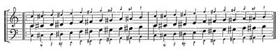
This auditory illusion resembles some similarity to the effect caused by barber-poles in american and british barber shops. In the case of the barber-poles, one image with colored stripes in diagonal is attached to a rotating cylinder and presented over and over in circles. The interesting thing about this process is that the cycle is difficult to perceive, and therefore, creates the illusion of the stripes ascending forever.
Similarly, the auditory illusion proposed by Shepard is nothing but an analogy in the auditory domain, presenting a cycle of raising harmonics that repeats every octave.
In order to achieve this auditory illusion, we could summarize the steps proposed by Shepard as following:
Computing several harmonics one octave apart from each other
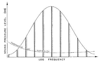
The harmonics in the middle must be louder than the ones at the beginning or end of the frequency spectrum
We need to change the gain of each harmonic as time goes on, for example, using some spectral envelope
Shepard achieves the change of gain for each harmonic by using a raised-cosine spectral envelope.
It is mainly this idea of the raised-cosine spectral envelope that has been preserved and reformulated in the audio effects proposed by Esqueda, Välimäki, and Parker. This type of effects have been called barber-pole flanging and phasing illusions, in accordance to the similarity to the barber-poles, mentioned before in the introduction.
Esqueda, Välimäki, and Parker present three different ideas for implementing barber-pole phasing and flanging audio effects: A network of cascaded time-varying notch filters, a synchronized dual flanger, and a single-sideband modulation filter.
In the following sections of this paper, I will briefly introduce the concept of each of these filters proposed by Esqueda, Välimäki, and Parker. Then, in the following section I am going to provide my experience implementing one of them, the network of cascaded time-varying notch filters.
Cascaded Time-Varying Notch Filters
In the original proposal by Shepard, the methodology considers the creation of the auditory illusion by means of the additive synthesis of several harmonics, which are one octave apart, and whose gain is shaped by the raised-cosine spectral envelope.
This and the other audio effects, however, are dealing with a different problem, which involves not the attempt to synthesize the illusion from scratch, but instead, having an input signal and filtering it in some way so the illusion emerges from the content of the signal itself.
Phasers and flangers work by creating sweeping notches in the spectrum of the original signal, these are the selected mechanisms by Esqueda, Välimäki, and Parker to create the barber-pole illusions.
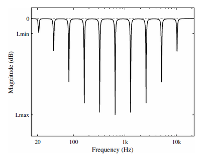
The magnitude of a network of cascaded notch-filters is presented.
Each notch in the magnitude response represents the contribution of a different notch-filter.
In general, this method of generating the auditory illusion is the one that feels the closest to the original proposal by Shepard. For Shepard, each harmonic represented an additional element in the chain of additive synthesis. By contrast, in this audio effect each notch-filter is an additional element in the network that shapes the spectrum of the original signal so that the barber-pole illusion emerges.
The level of gain of each notch-filter, in this case attenuation, is also controlled by a raised-cosine envelope, and time-varying for every sample of the signal.
Synchronized Dual Flanger
The second effect proposed by Esqueda, Välimäki, and Parker is a dual flanger.
The design of the system starts as a single flanger. The first interesting characteristic of this flanger is the decision of using a sawtooth waves as the Low-Frequency Oscillator (LFO) that modulates the gain of the delayed signal, as well as another sawtooth wave that modulates the length of the delay.
The motivation for using a sawtooth LFO is simple and elegant, it provides an unidirectional growth over time that abruptly restarts for the beginning of the next cycle. The auditory illusion requires that the sweeping of the notches moves in the same direction for the entire cycle, the sawtooth LFO provides exactly that.
One drawback introduced by this approach is the abrupt interruption introduced by restarting the cycle from one instant to another, which can give away the cyclic behavior of the system, and which is enemy to the purpose of creating the auditory illusion. In order to soften the transition between one cycle and another, the second flanger is added. Hence, the dual flanger system.
The second flanger is an identical copy of the first flanger, it also has a sawtooth LFO modulating the delay range and gain of the flanger, the main difference is that both LFOs are in a $\frac{pi}{2}$ phase with respect to their corresponding LFOs in the first flanger.
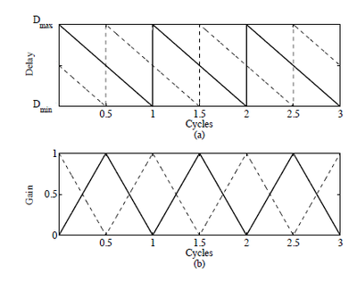
Figure 4 shows the phase relationship between the two flangers in the dual-flanger system.
Single-Sideband Modulation
The third method presented by Esqueda, Välimäki, and Parker consists of a system based on the combination of a signal and a frequency-shifted version of the same signal (single-sideband modulation).
Three main important considerations have to be addressed in the method proposed by Esqueda, Välimäki, and Parker. The first consideration is that the frequency-shifted copy of the signal should be added to the original signal only after delaying it for a short period. It is the short delay that generates the notches in the spectrum of the output signal of the system.
The second consideration is that it is necessary to have linearity between the frequency shifter and the delay given to the modulated signal. Once this two considerations are met, the system will produce notches that are linearly distributed across the spectrum and that sweep in the same direction.
Since the notches produced by the system are linearly distributed, this does not favor the emergence of the barber-pole illusion. In order for this to happen, the notches need to be one octave apart from each other, as in the method by Shepard.
The third consideration deals with this problem, Esqueda, Välimäki, and Parker suggest replacing the delay line of the system for a chain of first-order all-pass filters acting as an spectral delay.
With this final modification, the system is able to produce sweeping notches that are one octave from each other provided that the settings on each of the all-pass filters are accurately optimized to meet the desired group-delay curve.
Implementation of the cascaded time-varying notch-filters
The description of the systems presented by Esqueda, Välimäki, and Parker is informative regarding the methodologies that should be followed to accomplish an implementation of each of the systems.
Here we follow the methodologies proposed for the first system, the network of cascaded notch-filters, to implement a prototype of the audio effect in MATLAB.
The code of the implementation is given as an accompanying resource to this paper, the code consists of several functions that compute all of the parameters required for the system to operate on any given input signal. The accompanying implementation also provides two main scripts, one that provides an entry-point for the filter, which should be called to process an input signal, furthermore, another script tests and makes use of this entry-point with a white-noise signal and a combination of parameters that successfully create a barber-pole auditory illusion.
The first step in the process of implementing this audio effect is to separate the global parameters of the system from the time-varying parameters, i.e., the parameters that should be computed every short-time (in practice, every sample) in which the filter is operating.
This division between global and time-varying parameters is not given by the original proposal of Esqueda, Välimäki, and Parker. Therefore, it represents an interpretation of the parameters and workflow of the original methodology that must be made in order to effectively implement a prototype of the working system.
The global parameters of the audio effect are the following:
$M$: The number of notch-filters in the cascade
$F_s$: The sampling rate of the system
$K$: The number of frequencies per cycle. Given by $K = \text{floor}(F_s/p)$
$Q$: A control of the bandwidth of the notch-filters
$p$: The repetition rate of the cycle (how many times is the system reaching an octave every second), in Hertz
$L_{min}$: Minimum loudness level, in decibels
$L_{max}$: Maximum loudness level, in decibels
The time-varying parameters of the audio effect are the following:
$f_c(m,k)$: Center frequency of the $m^{th}$ filter in the $k^{th}$ frequency index of the cycle
$L_c(m,k)$: Loudness of the $k^{th}$ frequency of the $m^{th}$ filter, in decibels
$G$: The normalized version of gain $L_c$, in the range $[0,1]$
$\beta$: A factor that involves the bandwidth and the gain at the bandwidth, used to compute the coefficients of the notch-filters
Once the most important parameters of the system have been defined and classified accordingly, the next step is to define the workflow of the system, especially for the time-varying part of the system which is the most complicated to implement, as it involves the computation of the coefficients for all of the filters involved in the network.
Given that the parameter $K$ dictates the number of frequencies that have to be computed every cycle, this parameter defines the length of the short-time sections of the signal that have to be processed by the system. In fact, using the definition provided by Esqueda, Välimäki, and Parker for computing the value of $K$, we can observe that it is equivalent to the number of samples that exist in one cycle. This means that there is a relationship of one sample for one frequency in every case, for any sampling rate or repetition rate of the system. At this point, we can safely assume that our implementation of the audio effect has to effectively compute a new set of notch-filters for every sample of the input signal.
The implementation that we followed, considers then, that the global parameters will be provided by the user to the system. One exception are the global parameters which can be obtained from other global parameters (e.g., $K$), these are not required from the user and are computed internally instead.
Once the global parameters are present in the system, we then start processing the signal.
The methodology from Esqueda, Välimäki, and Parker provides the transfer function used to compute each of the notch-filters of the system.
$$H(z) = \frac{ \big( \frac{ 1 + g \beta }{ 1 + \beta } \big) - 2 \big( \frac{ \cos( \frac{ 2 \pi f_c }{ F_s } ) }{ 1 + \beta } \big) z^{-1} + \big( \frac{ 1 - G \beta }{ 1 + \beta } \big) z^{-2} }{ 1 - 2 \big( \frac{ \cos( \frac{ 2 \pi f_c }{ F_s } ) }{ 1 + \beta } \big) z^{-1} + \big( \frac{ 1 - \beta }{ 1 + \beta } \big) z^{-2} } $$
The most efficient way to compute the network of cascaded notch-filters would be to anticipate the system by multiplying the transfer function of a network of notch-filters to get one resulting system and use this system to filter the input signal, however, since the number of notch-filters in our network is an unknown parameter, $M$, controlled by the user, it is not easy to come with a strategy to pre-compute all the possible numbers of notch-filters in the network and their combinations with different parameters, such as the rate of the cycle of the audio effect.
Therefore, I have decided that it is probably an easier strategy to use this transfer function to go back to the difference equation of the system, and compute the pertinent values of the coefficients of the system as they are needed.
The difference equation of a notch-filter is the following:
$$y[n] = b_0 x[n] - b_1 x[n-1] + b_2 x[n-2] + a_1 y[n-1] - a_2 y[n-2]$$
Where the coefficients of the system correspond to
$$b_0 = \frac{ 1 + G \beta }{ 1 + \beta }$$
$$b_1 = \frac{ 2 \cos( \frac{ 2 \pi f_c }{ F_s }) }{ 1 + \beta }$$
$$b_2 = \frac{ 1 - G \beta }{ 1 + \beta }$$
$$a_1 = b_1$$
$$a_2 = \frac{ 1 - \beta }{ 1 + \beta }$$
The final implementation consists then of a delay-line of second order which filters the input signal through a cascade of $M$ notch-filters. The coefficients of the notch-filters are computed for every sample, according to the properties of each notch-filter, namely, their center frequency $f_c$ and the attenuation computed for that center frequency $(L_c, G)$.
The implementation was done in Matlab, and all the source code is available here.
As an example, here is an audio input to the system and what it comes out.
Input [wav]
Output [wav]
Conclusions
In this paper, I outline the implementation of a cascaded notch-filter system to create auditory illusions from an input signal. The reference methodology by Esqueda, Välimäki, and Parker was very informative about the parameters, formulas and methodologies used to test the filter and generate the sound samples and the plots presented in their paper. The implementation proposed here used the transfer function presented in the reference methodology and used it to get the difference equation of a notch-filter, computing its parameters for every sample and using those coefficients to filter the input signal through a delay-line of second order.