MUMT 618: Implementation of Boss DS-1

MATLAB implementation of a digital model of distortion by Yeh et al. (2007).

Abstract

This is a report for my final project of the MUMT 618: Computational Modeling of Musical Acoustic Systems class at McGill University.

I will describe my experience implementing a digital model of distortion that has been presented in the paper titled “Simplified, physically-informed models of distortion and overdrive guitar effects pedals”, presented in 2007 by David Yeh, Jonathan Abel, and Julius Smith at the DAFx'07 Conference.

Although this paper describes two models:

1. Boss DS-1, a distortion pedal
2. Ibanez TS-9, an overdrive pedal

I have only implemented the model of the Boss DS-1 distortion pedal. The implementation provided has been done in MATLAB and does not opertate in real-time, however, a real-time implementation should not be difficult to derivate from the given code. I also provide a few audio examples of the audio effect. As of my knowledge, there are no existing audio examples or code for this model previous to this write-up, therefore, I consider it is a valuable contribution for anyone following the ideas of this paper for reproducing or improving the model.

Overview

A high-level overview can be seen in the following diagram from the paper

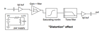
It is possible that all of these stages may have an audible effect in the output produced by the physical pedal, however, the model only provides a continuous-time transfer function for the Gain + filter and the Saturating nonlin stages, therefore, this implementation concentrates in these two stages only.

The diagrams presented in the paper are excerpts of the circuit, which are sometimes difficult to follow, therefore, as an additional resource, it was very helpful to consult this article from ElectroSmash. In this document, a full view of the schematic is displayed with the different stages labeled.

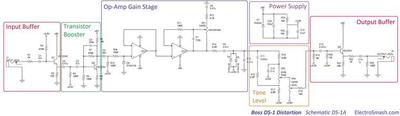
The Gain + filter stage in the paper’s diagram corresponds to the Transistor Booster stage of the schematic, its main component is a bipolar junction transistor. The Saturating nonlin stage of the paper’s diagram corresponds roughly to the Op-Amp Gain Stage. From now on, I will refer to the names of the schematic as I find them more intuitive.

Transistor Booster Stage

This stage corresponds to a single bipolar junction transistor, the continuous-time transfer function provided in the paper is the following:

$$ H(s) = \frac{s^{2}}{(s + \omega_1) (s + \omega_2)} $$

where $ \omega_1 = 2\pi3 $ and $ \omega_2 = 2\pi600 $

Op-Amp Gain Stage

This stage corresponds to the main nonlinearity of the circuit, according to the paper. One parameter is provided in this stage to control the amount of distortion that the audio effect will output. The continuous-time transfer function is defined as following:

$$ H(s) = \frac{(s + \frac{1}{R_t C_c}) (s + \frac{1}{R_b C_z}) + \frac{s}{R_b C_c}}{(s + \frac{1}{R_t C_c})(s + \frac{1}{R_b C_z})} $$

where $$R_t = 100 000 D $$ $$R_b = (1-D)100 000 + 4700$$ $$C_z = 0.000 001$$ $$C_c = 0.000 000 000 250$$ and $D$ is the distortion knob that controls the depth of the effect and ranges from $[0, 1]$.

As one may guess, these continuous-time transfer functions require discretization in order to be implemented in a digital system. In order to discretize them, Yeh et al. propose the use of the bilinear transform. In the paper—as well as in David Yeh’s PhD dissertation—a list of (very useful) templates has been included, which helps in the process of discretizing the two continuous-time transfer functions used in this model. The relevant templates for this implementation are the templates corresponding to second-order filters.

Bilinear Transform

In order to discretize a continuous-time transfer function, first, we should put the continuous-time transfer function in the following form $$ H(s) = \frac{b_2 s^2 + b_1 s + b_0}{a_2 s^2 + a_1 s + a_0} $$

Once we compute the corresponding coefficients, they can be placed in a discrete-time transfer function of the form

$$ H(z) = \frac{B_0 + B_1 z^{-1} + B_2 z^{-2}}{A_0 + A_1 z^{-1} + A_2 z^{-2}} $$

The discrete-time coefficients of this transfer function can be obtained from the following equations $$ B_0 = b_0 + b_1 c = b_2 c^2 $$ $$ B_1 = 2b_0 - 2b_2 c^2 $$ $$ B_2 = b_0 - b_1 c = b_2 c^2 $$ $$ A_0 = a_0 + a_1 c = a_2 c^2 $$ $$ A_1 = 2a_0 - 2a_2 c^2 $$ $$ A_2 = a_0 - a_1 c = a_2 c^2 $$

After plugging the coefficients into the discrete-time transfer function, we should be able to implement the resulting transfer function as a digital filter.

Implementation of the Transistor Booster Stage

Using the steps described above, I now describe the implementation of the Transistor Booster Stage part of the model.

The first step would be to put the given continuous-time transfer function in the form of the bilinear transform template $$ H(s) = \frac{s^2}{s^2 + (\omega_1 + \omega_2)s + \omega_1 \omega_2} $$ From here, the continuous-time coefficients can be easily extracted $$ b_2 = 1 $$ $$ b_1 = 0 $$ $$ b_0 = 0 $$ $$ a_2 = 1 $$ $$ a_1 = \omega_1 + \omega_2 = 2\pi 3 + 2\pi 600 = 1206\pi $$ $$ a_0 = \omega_1 \omega_2 = (2\pi 3)(2 \pi 600) = 7200\pi^2 $$

Working the templates for the discrete-time coefficients results in the following $$ B_0 = 4fs^2 $$ $$ B_1 = -8fs^2 $$ $$ B_2 = 4fs^2 $$ $$ A_0 = 7200\pi^2 + 2412\pi fs + 4fs^2 $$ $$ A_1 = 14400\pi^2 - 8fs^2 $$ $$ A_2 = 7200\pi^2 - 2412\pi fs + 4fs^2 $$

Showing once again the template of the second-order discrete-time transfer function $$ H(z) = \frac{B_0 + B_1 z^{-1} + B_2 z^{-2}}{A_0 + A_1 z^{-1} + A_2 z^{-2}} $$

Plugging the values of the coefficients recently found, gives the following equation $$ {\scriptsize H(z) = \frac{4fs^2 - 8fs^2 z^{-1} + 4fs^2 z^{-2}}{(7200\pi^2 + 2412\pi fs + 4fs^2) +(14400\pi^2 - 8fs^2) z^{-1} + (7200\pi^2 - 2412\pi fs + 4fs^2) z^{-2}}} $$

After dividing by $4$, factorizing $fs$, and doing some algebra to simplify the equation, this can be expressed as: $$ {\small H(z) = \frac{1 -2 z^{-1} + z^{-2}}{(1800 \Omega^2 + 603 \Omega + 1) + (3600 \Omega^2 - 2) z^{-1} + (1800\Omega^2 - 603\Omega + 1) z^{-2}} } $$

with $\Omega = \frac{\pi}{fs}$

The implementation of this discrete-time transfer function results in a filter with the following magnitude response:

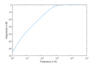
By inspecting the original magnitude response shown in the paper, it can be concluded that the implemented filter should output above $30dB$ of gain in its bandpass.

Luckily, in the corresponding section of this stage, the paper mentions that the expected gain in the bandpass is, in fact, $36dB$. Using this information, an additional gain, $g$, is included in the discrete-time transfer function:

$$ {\small H(z) = \frac{g(1 -2 z^{-1} + z^{-2})}{(1800 \Omega^2 + 603 \Omega + 1) + (3600 \Omega^2 - 2) z^{-1} + (1800\Omega^2 - 603\Omega + 1) z^{-2}} } $$

where the equation, $36dB = \log_{10}(g) * 20$, can be used to obtain the value of $g$

$$ g = 10^{\frac{36}{20}} = 63.0957 $$

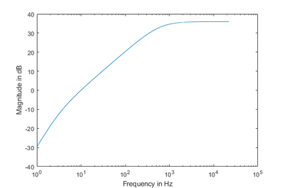
The resulting magnitude response resembles much more the magnitude response shown in the paper

This filter—including its correction—can be implemented with the following MATLAB function:

% Transistor Booster Stage
% Implementation by Nestor Napoles Lopez
% based on the paper by Yeh et al. (2007)

function y = bjtfilt(x, fs)

% After working the math, I put all the discrete-time
% coefficients in terms of this variable coeff
coeff = pi/fs;

B0 = 1;
B1 = -2;
B2 = 1;

A0 = 1800.*coeff.^2 + 603.*coeff + 1;
A1 = 3600.*coeff.^2 - 2;
A2 = 1800.*coeff.^2 - 603.*coeff + 1;

% We obtain the gain from
% 36dB = log10(x) * 20
amp = 10.^(36/20);
B = amp .* [B0, B1, B2];
A = [A0, A1, A2];

y = filter(B, A, x);

end

Implementation of the Op-Amp Gain Stage

Just as done during the Transistor Booster Stage, the implementation of the Op-Amp Gain Stage starts from a given continuous-time transfer function $$ H(s) = \frac{(s + \frac{1}{R_t C_c}) (s + \frac{1}{R_b C_z}) + \frac{s}{R_b C_c}}{(s + \frac{1}{R_t C_c})(s + \frac{1}{R_b C_z})} $$

Putting this transfer function in the form of the bilinear transform template $$ H(s) = \frac{s^2 + (\frac{1}{R_b C_z} + \frac{1}{R_t C_c} + \frac{1}{R_b C_c})s + \frac{1}{R_t C_c R_b C_z}}{s^2 + (\frac{1}{R_b C_z} + \frac{1}{R_t C_c})s + \frac{1}{R_t C_c R_b C_z}} $$

The continous-time coefficients can be obtained $$ b_2 = 1 $$ $$ b_1 = \frac{1}{R_b C_z} + \frac{1}{R_t C_c} + \frac{1}{R_b C_c} $$ $$ b_0 = \frac{1}{R_t C_c R_b C_z} $$ $$ a_2 = 1 $$ $$ a_1 = \frac{1}{R_b C_z} + \frac{1}{R_t C_c} $$ $$ a_0 = \frac{1}{R_t C_c R_b C_z} $$

Some of these coefficients are equivalent (e.g., $a_0 = b_0$), therefore, they can be summarized in the following coefficients: $$ ab_2 = 1 $$ $$ a_1 = \frac{1}{R_b C_z} + \frac{1}{R_t C_c} $$ $$ b_1 = a_1 + \frac{1}{R_b C_c} $$ $$ ab_0 = \frac{1}{R_t C_c R_b C_z} $$

The next step is to obtain the discrete-time coefficients, these can be expressed in terms of the simplified list of continuous-time coefficients presented above: $$ B_0 = ab_0 + b_1 c + c^2 $$ $$ B_1 = 2ab_0 - 2c^2 $$ $$ B_2 = ab_0 - b_1 c + c^2 $$ $$ A_0 = ab_0 + a_1 c + c^2 $$ $$ A_1 = 2ab_0 - 2c^2 $$ $$ A_2 = ab_0 - a_1 c + c^2 $$

In this case, the resulting magnitude response

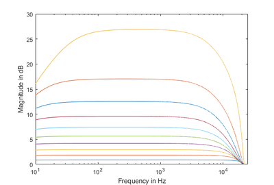
is quite similar to the magnitude response shown in the paper

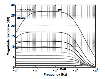
The different colors of the first plot represent the magnitude response with values of $D$ going from $0.1$ to $1.0$. This is the MATLAB function that implements this filter:

% Op-Amp Gain Stage
% Implementation by Nestor Napoles Lopez
% based on the paper by Yeh et al. (2007)

function y = opampfilt(x, fs, DIST)

% Resistors and capacitors from the model
Rt = 100000 * DIST;
Rb = 100000*(1-DIST) + 4700;
Cz = 0.000001;
Cc = 0.000000000250;

% Constant for the bilinear transform
c = 2*fs;

% Continuous-time coefficients (reduced)
ab0 = 1 / (Rt*Cc*Rb*Cz);
a1 = 1/(Rb*Cz) + 1/(Rt*Cc);
b1 = a1 + 1/(Rb*Cc);

% Discrete-time coefficients
B0 = ab0 + b1*c + c.^2;
B1 = 2*ab0 - 2*c.^2;
B2 = ab0 - b1*c + c.^2;

A0 = ab0 + a1*c + c.^2;
A1 = B1;
A2 = ab0 - a1*c + c.^2;

B = [B0, B1, B2];
A = [A0, A1, A2];

y = filter(B, A, x);

end

Diode-Clipper

At the end of the Op-Amp Gain Stage, there is an additional step that simulates the diode that clips the samples exceeding a gain threshold, in the case of the digital implementation, that threshold consists of $abs(x[n]) \geq 1.0$. The diode-clipper has been implemented using one of the proposed methods in the paper:

$$ \text{clipper}(x) = \frac{x}{(1 + |x|^n)^{1/n}} $$

with $n = 2.5$

The MATLAB code for the clipping function is the following:

% Diode clipper
% Implementation by Nestor Napoles Lopez, December 2018
% based on the paper by Yeh et al. (2007)

function x = diodeclip(x)

n = 2.5;

for i=1:length(x)
    x(i) = x(i) / (1 + abs(x(i)).^n).^(1/n);
end

end

As a final step, I provide a script that cascades the two stages of the models to process an input audio example:

% DS-1, main script
% Implementation by Nestor Napoles Lopez, December 2018
% based on the paper by Yeh et al. (2007)

% Sample audio
[x, fs] = audioread('guitar_clean.wav');

% Bipolar Junction Transistor Stage
y = bjtfilt(x, fs);

% Op-amp Gain Stage
D = 1; % D lies between [0, 1]
y = opampfilt(y, fs, D);

% Diode clipper
y = diodeclip(y);

s = audioplayer(y, fs);
play(s);

Here is an example of the model applied to an audio sample of a clean electric guitar¹:

Original audio [wav]

Transistor Booster Stage only [wav]

Op-Amp Gain Stage only [wav]

Transistor Booster Stage and Op-Amp Gain Stage [wav]