MUMT 621: Hidden Markov Model for Symbolic Key Detection

A Hidden Markov Model (HMM) for retrieving the musical key of a MIDI file.

Abstract

During the course MUMT 621: Music Information Acquisition, Preservation, and Retrieval, I designed and implemented a model for symbolic key detection.

The model was later extended to work with audio data and to retrieve local-key estimations as well. A dedicated entry in this website exists for the extended version, which was published in the proceedings of DLfM 2019.

This document describes the original class project. A PDF version of this document is also available.

Introduction

Finding the key of a piece of Western art music has been in the interest of the Music Information Retrieval (MIR) community for several years already. Since they were introduced, the design or acquisition of key-profiles have been the preferred methodology to solve this problem. In this project, we combine the use of key-profiles with the capabilities of Hidden Markov Models (HMMs) to model the time-varying aspects of music to find the key of a piece of music by considering the pitch-class of every note in the piece as the observation symbol of an HMM.

Design of the Hidden Markov Model

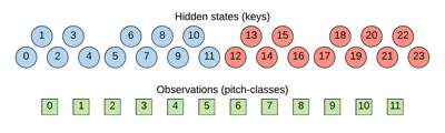
As mentioned, the proposed HMM consists of 24 hidden states and 12 observation symbols.

Keys as hidden states

The hidden states correspond to 24 different major and minor keys (i.e., no distinction between enharmonics), each of these keys is represented as a hidden state in the model. All of the keys may transition to any of the other 23 keys, however, the probability of transitioning to neighbor keys in the circle of fifths is preferred over distant keys.

Pitch-classes as observation symbols

All major and minor keys are able to emit any of the twelve pitch-classes before they transition to a new state, however, by acquiring the probability distributions from common key-profiles used for the task of key detection, the emission of diatonic tones of the key are preferred over accidental tones.

Parameters of the model

Initial probabilities

The initial probabilities of the model are the same for each key, $p(state) = \frac{1}{24}$.

State transitions

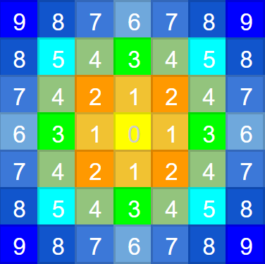
The probability distributions for state transitions that happen after the initialization have been taken from a geometric model of key distance. The probability of a transition to another key in the next group of neighbors decreases exponentially. The geometric model of key distance can be observed in

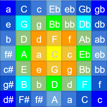
Using this model, we can observe, for example, a list of the groups of neighbor keys for C Major, in descending order:

Group   Keys
0       C
1       G F a c
2       d e f g
3       D Eb A Bb
4       E Ab bb b
5       Db B
6       eb f#
7       c# ab
8       F#

This structure of nine groups of neighbours repeats for all major and minor keys. We can use these groups to compute the transition probability for any key according to the following formula:

$$p(s) = \alpha^{(G-1) - s_g}$$

where $G$ is the number of groups of neighbor keys to the current tonic, according to the geometric model (i.e., $G=9$), $s_g$ is the group to which the key $s$ belongs, $\alpha$ is the probability ratio between a key of one group and a key from a contiguous group.

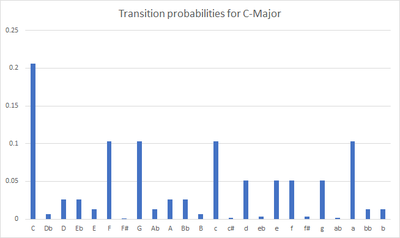
Figure 4 shows a plot of the probability distribution for the transition to the next key, if the current key is C Major.

Emission probabilities

The emission probability distributions have been taken from the common key-profiles used by other key detection algorithms. Particularly, we considered the same five pairs of key-profiles used in the comparison by Albrecht and Shanahan (2013).

Dataset

The model has been evaluated using sets of short musical compositions in all major and minor keys. Each set follows the format of the Well-Tempered Clavier by Johann Sebastian Bach. The sets are: The Well-Tempered Clavier, Volume I, by Johann Sebastian Bach (24 MIDI files); The Well-Tempered Clavier (Part II), by Johann Sebastian Bach (24 MIDI files); Preludes Op.28, by Frédéric Chopin (24 midi files); 4 of the 24 preludes from Op.11, by Alexander Scriabin (4 MIDI files); Preludes and Fugues Op.87, by Dmitri Shostakovich (48 MIDI files). In total, 124 MIDI files were used for testing the algorithm.

Even if these MIDI files have not been explicitly annotated with their keys and modulations, the main key of each of the selected pieces has been clearly established by the composer in the original scores, meaning an evaluation process of the algorithm is possible at least against the main key of the musical piece.

Results

The best performance of the algorithm used a ratio of $\alpha = 10$, the key-profiles from Temperley for major keys, and the key-profiles from Sapp for minor keys. With this configuration, the algorithm guessed correctly 103 out of 124 keys in the MIDI files from the dataset.

The worst performance of the algorithm used a ratio of $\alpha = 2$, the key-profiles from Krumhansl and Kessler for major keys, and the key-profiles from Aarden and Essen for the minor keys. With this configuration, the algorithm guessed 49 out of 124 keys in the MIDI files from the dataset.